Run an AI algorithm on GPUs
Introduction
This tutorial aims to run an AI algorithm in python on computational clusters. It is composed of two parts:
- launching the training of an AI model on the Bigfoot cluster using a submission script.
- launch a Jupyter Notebook to load the previously trained model and run it with an interactive job
Prerequisites
- Be connected to the Bigfoot cluster front-end with your login/password.
- Have a local ssh configuration with transparent proxy.
If this is not yet the case, click here.
Linux bigfoot 5.10.0-14-amd64 #1 SMP Debian 5.10.113-1 (2022-04-29) x86_64
                       Welcome to Bigfoot cluster!

                             :            :
                            .'            :
                        _.-"              :
                    _.-"                  '.
    ..__...____...-"                       :
   : \_\                                    :
   :    .--"                                 :
   `.__/  .-" _                               :
      /  /  ," ,-                            .'
     (_)(`,(_,'L_,_____       ____....__   _.'
      "' "             """""""          """

GPU, GPU, GPU, ... ;-)

            Type 'chandler' to get cluster status
          Type 'recap.py' to get cluster properties

Sample OAR submissions:
  # Get a A100 GPU and all associated cpu and memory resources:
  oarsub -l /nodes=1/gpu=1 --project test -p "gpumodel='A100'" "nvidia-smi -L"
  # Get a MIG partition of an A100 on a devel node, to make some tests
  oarsub -l /nodes=1/gpu=1/migdevice=1 --project test -t devel "nvidia-smi -L"

Last login: Fri Jul 22 15:38:45 2022 from 129.88.178.43
login@bigfoot:~$
Launching a training
In this part, the goal is to launch the training of an artificial intelligence model on the Bigfoot computing cluster via a submission script.
Python environment
First of all, you have to choose your working environment, which must include Python and the necessary modules. For the management of Python modules we will use conda.
The following script is used to source conda:
login@bigfoot:~$ source /applis/environments/conda.sh
Then you just have to choose one of the conda environments available on Bigfoot.
The following command displays the different environments available:
login@bigfoot:~$ conda env list
# conda environments:
#
base                  *  /applis/common/miniconda3
GPU                      /applis/common/miniconda3/envs/GPU
f-ced-gpu                /applis/common/miniconda3/envs/f-ced-gpu
fidle                    /applis/common/miniconda3/envs/fidle
fidle-orig               /applis/common/miniconda3/envs/fidle-orig
gpu_preprod              /applis/common/miniconda3/envs/gpu_preprod
julia                    /applis/common/miniconda3/envs/julia
tensorflow1.x_py3_cuda10.1     /applis/common/miniconda3/envs/tensorflow1.x_py3_cuda10.1
tensorflow2.x_py3_cuda10     /applis/common/miniconda3/envs/tensorflow2.x_py3_cuda10
torch1.x_py3_cuda10      /applis/common/miniconda3/envs/torch1.x_py3_cuda10
torch1.x_py3_cuda92      /applis/common/miniconda3/envs/torch1.x_py3_cuda92
In our example we will choose the GPU environment which contains all the modules necessary to use TensorFlow/Keras and PyTorch.
The following command displays all the modules available in a given environment.
login@bigfoot:~$ conda list -n GPU
It is not possible to add a module to one of the environments proposed above or to modify their versions.
It is possible to create your own environment if a necessary module is not present in the proposed environments. For more information about conda, go to this page
Training program
In this example, we will build a basic classification network of the MNIST DataSet and train it.
Let’s start by moving to our dedicated directory on the Bettik storage service by replacing login with your Perseus ID in the following command, and project_name by a project you are a member of :
login@bigfoot:~$ cd /bettik/PROJECTS/project_name/login
To create the classification network, we need to create a train.py file in a tuto_ia/ directory containing the following code:
import tensorflow as tf

from tensorflow.keras.datasets import mnist
from tensorflow.keras.utils import to_categorical

from tensorflow.keras import Input
from tensorflow.keras.layers import Dense, Activation
from tensorflow.keras.models import Model

from tensorflow.python.client import device_lib
print("GPUs Available: ", tf.config.experimental.list_physical_devices('GPU'))

(X_train, y_train), (X_test, y_test) = mnist.load_data()
num_train  = X_train.shape[0]
img_height = X_train.shape[1]
img_width  = X_train.shape[2]
X_train = X_train.reshape((num_train, img_width * img_height))
y_train = to_categorical(y_train, num_classes=10)

num_classes = 10
xi      = Input(shape=(img_height*img_width,))
xo      = Dense(num_classes)(xi)
yo      = Activation('softmax')(xo)
model   = Model(inputs=[xi], outputs=[yo])

model.compile(loss='categorical_crossentropy',
              optimizer='adam',
              metrics=['accuracy'])

callbacks = [tf.keras.callbacks.ModelCheckpoint(
              filepath="best_model.h5",
              monitor='val_accuracy',
              mode='max',
              save_best_only=True)]

model.fit(X_train, y_train,
          batch_size=128,
          epochs=20,
          verbose=1,
          validation_split=0.1,
          callbacks=callbacks)
import torch
import torch.nn as nn
from torchvision import datasets, transforms
from tqdm import tqdm
import sys

class Classifier(nn.Module):
    def __init__(self):
        super(Classifier, self).__init__()
        self.linear = nn.Linear(in_features=28*28, out_features=10)
        self.activation = nn.Softmax(dim=1)

    def forward(self, x):
        x = self.linear(x)
        output = self.activation(x)
        return output

def train(model, device, train_loader, val_loader, optimizer, epochs):
    prev_acc = 0
    for epoch in range(epochs):
        print(f"Epoch {epoch+1}/{epochs}")
        model.train()
        for batch in tqdm(train_loader, file=sys.stdout):
            X, Y = batch
            X, Y = X.to(device), Y.to(device)
            Y_pred = model(X)
            optimizer.zero_grad()
            loss = nn.CrossEntropyLoss()(Y_pred, Y)
            loss.backward()
            optimizer.step()
        model.eval()
        with torch.no_grad():
            accuracy = 0
            for (X, Y) in val_loader:
                X, Y = X.to(device), Y.to(device)
                y_pred = model(X)
                y_classes = torch.argmax(y_pred, dim=1)
                accuracy += torch.sum(y_classes == Y)
            accuracy = accuracy.item()/len(val_loader.dataset)
            print(f"Validation accuracy : {accuracy}")
            if accuracy > prev_acc:
                torch.save(model, "best_model.pt")
            prev_acc = accuracy

def main():
    use_cuda = torch.cuda.is_available()
    device = torch.device("cuda" if use_cuda else "cpu")
    print(f"Used device : {device}")

    transform=transforms.Compose([
        transforms.ToTensor(),
        torch.squeeze,
        torch.flatten
    ])

    dataset = datasets.MNIST("data", train=True, download=True, transform=transform)
    train_size = int(0.8 * len(dataset))
    val_size = len(dataset) - train_size
    train_dataset, val_dataset = torch.utils.data.random_split(dataset, [train_size, val_size])
    train_loader = torch.utils.data.DataLoader(train_dataset, batch_size=128)
    val_loader = torch.utils.data.DataLoader(val_dataset, batch_size=128)

    model = Classifier().to(device)
    adam = torch.optim.Adam(model.parameters(), lr=0.01)

    train(model, device, train_loader, val_loader, adam, 20)

if __name__ == "__main__":
    main()
To do this, you can either create the train.py file containing this code directly on the cluster, or create it on your local machine and transfer it to your Bettik space with the following command by replacing login with your Perseus ID:
local-login@local-computer:~$ rsync -avxH train.py login@cargo.univ-grenoble-alpes.fr:/bettik/PROJECTS/project_name/login/tuto_ia/
This small python program creates the classification model, trains it on a training dataset, display its progress on the standard output, and saves the best model in the tuto_ia/ directory.
Write an execution script
Once the training program is ready, you have to write a script to submit the launch of a job on the computing machines.
To do this, simply create a run_train.sh file containing the following code, and replace login by your Perseus ID and project_name by your project name:
#!/bin/bash

#OAR -n tuto_training
#OAR -l /nodes=1/gpu=1,walltime=0:30:00
#OAR --stdout %jobid%.out
#OAR --stderr %jobid%.err
#OAR --project project_name
#OAR -p gpumodel='V100'

cd /bettik/PROJECTS/project_name/login/tuto_ia
source /applis/environments/cuda_env.sh bigfoot 10.2
source /applis/environments/conda.sh
conda activate GPU

python train.py
This script allows you to prepare the OAR request by specifying the resources needed, the project concerned, or the management of standard inputs and outputs.
Details of the OAR commands are available here
It also prepares the necessary conda and cuda environments, and runs the model training.
Submit the job
We can now launch the job on the computing machines.
First, we have to make the script executable with the following command :
login@bigfoot:/bettik/PROJECTS/project_name/login/tuto_ia/$ chmod +x run_train.sh
We can then submit its execution via the resource manager with the command :
login@bigfoot:/bettik/PROJECTS/project_name/login/tuto_ia$ oarsub -S ./run_train.sh
[ADMISSION RULE] Modify resource description with type constraints
OAR_JOB_ID=18545
The job has been submitted and an ID has been assigned to it: OAR_JOB_ID=18545
Follow the execution of the job
We can now follow the progress of our job using a few commands by replacing login by your Perseus ID :
login@bigfoot:/bettik/PROJECTS/project_name/login/tuto_ia$ oarstat -u login
Job id    S User     Duration   System message
--------- - -------- ---------- ------------------------------------------------
18545     W login       0:00:00 R=32,W=0:30:0,J=B,N=Entrainement_tuto,P=your-project (Karma=0.014,quota_ok)
We can see that the job is waiting for resources, in fact its status is W for Waiting. You will have to wait until the requested resource is available.
If we try again later, we obtain :
login@bigfoot:/bettik/PROJECTS/project_name/login/tuto_ia$ oarstat -u login
Job id    S User     Duration   System message
--------- - -------- ---------- ------------------------------------------------
18545     R login       0:00:13 R=32,W=0:30:0,J=B,N=Entrainement_tuto,P=your-project (Karma=0.014,quota_ok)
We see that the job has been running for 13 seconds, its status is R for Running.
The evolution of the standard output of your algorithm can be followed with the following command (replacing 18545 by the ID of your job):
login@bigfoot:/bettik/PROJECTS/project_name/login/tuto_ia$ tail -f 18545.out
Epoch 1/20
54000/54000 [==============================] - 2s 32us/sample - loss: 13.1363 - accuracy: 0.7976 - val_loss: 4.3970 - val_accuracy: 0.8908
Epoch 2/20
54000/54000 [==============================] - 1s 15us/sample - loss: 4.9776 - accuracy: 0.8747 - val_loss: 3.5514 - val_accuracy: 0.9047
The model is now trained, and it is saved in the tuto_ia/ directory.
Exploiting the model
In this part, the goal is now to use an interactive job in order to launch a Jupyter Notebook on the cluster and access it from the browser of your local computer to load the model and evaluate it.
Launch a job interactively
Launching a job interactively allows you to access the terminal of a compute node to execute step by step commands. Once connected to the bigfoot cluster front-end, you just have to launch the following command:
login@bigfoot:~$ oarsub -I -l /nodes=1/gpu=1,walltime=1:00:00 -p "gpumodel='V100'" --project your-project
[ADMISSION RULE] Modify resource description with type constraints
OAR_JOB_ID=18584
Interactive mode: waiting...
Starting...
Connect to OAR job 18584 via the node bigfoot5
login@bigfoot5:~$
The arguments of this command are very similar to the ones given previously in the job submission script, they do exactly the same thing. However, we add here the -I option allowing to launch the job in Interactive mode.
In our example, the resource manager has connected us to bigfoot5.
Start the Jupyter Notebook server
Before starting the Jupyter Notebook, you must activate the necessary environments via the following commands:
login@bigfoot5:~$ source /applis/environments/cuda_env.sh bigfoot 10.2
login@bigfoot5:~$ source /applis/environments/conda.sh
login@bigfoot5:~$ conda activate GPU
(GPU) login@bigfoot5:~$
So now we can go to the right directory and start a Jupyter Notebook :
(GPU) login@bigfoot5:~$ cd /bettik/PROJECTS/project_name/login/tuto_ia/
(GPU) login@bigfoot5:/bettik/PROJECTS/project_name/login/tuto_ia$ jupyter notebook --no-browser --ip=0.0.0.0 &
[1] 23557
[I 10:25:56.965 NotebookApp] JupyterLab extension loaded from /applis/common/miniconda3/envs/GPU/lib/python3.7/site-packages/jupyterlab
[I 10:25:56.965 NotebookApp] JupyterLab application directory is /applis/common/miniconda3/envs/GPU/share/jupyter/lab
[I 10:25:56.968 NotebookApp] Serving notebooks from local directory: /home/login/tuto_ia
[I 10:25:56.968 NotebookApp] The Jupyter Notebook is running at:
[I 10:25:56.968 NotebookApp] http://(bigfoot5 or 127.0.0.1):8888/?token=452db8f89bfd209a9245662ed808f115cb666c1d15222cf3
[I 10:25:56.968 NotebookApp] Use Control-C to stop this server and shut down all kernels (twice to skip confirmation).
[C 10:25:57.004 NotebookApp]

    To access the notebook, open this file in a browser:
        file:///home/login/.local/share/jupyter/runtime/nbserver-23557-open.html
    Or copy and paste one of these URLs:
        http://(bigfoot5 or 127.0.0.1):8888/?token=452db8f89bfd209a9245662ed808f115cb666c1d15222cf3
The Jupyter Notebook is now running in the background of the cluster, so the terminal where the Notebook was launched is still accessible. As indicated, the Notebook server is accessible on the 8888 port of bigfoot5
To stop the Notebook server at the end of its use, use the command: jupyter notebook stop
Accessing the Jupyter Notebook from your local machine
To access this server from your local machine, you have to create an ssh tunnel between your machine and the cluster. To do so, you just have to run on your local computer the command :
local-login@local-computer:~$ ssh -fNL 8889:bigfoot5:8888 bigfoot.ciment
Of course, you have to adapt this command to your case:
- replace 8889 by any available port on your local machine
- replace bigfoot5 by the name of the machine on which the Notebook is launched
- replace 8888 by the port specified by Jupyter when launching the Notebook
- replace bigfoot.cement with what you have defined for transparent access in your ssh configuration
Once this command is executed, you have to access the Notebook from one of the browsers of your local machine at the address : http://localhost:8889, where 8889 is the port on your local machine chosen earlier.
When you first connect via a browser on each cluster, you will need to copy and paste the connection token provided by Jupyter when you launch the server:
[I 10:25:56.968 NotebookApp] The Jupyter Notebook is running at:
[I 10:25:56.968 NotebookApp] http://(bigfoot5 or 127.0.0.1):8888/?token=452db8f89bfd209a9245662ed808f115cb666c1d15222cf3
Here, you will have to copy and paste 452db8f89bfd209a9245662ed808f115cb666c1d15222cf3, in the browser token field.
Exploiting the model
Now you have to create a Jupyter notebook via the Jupyter graphical interface:
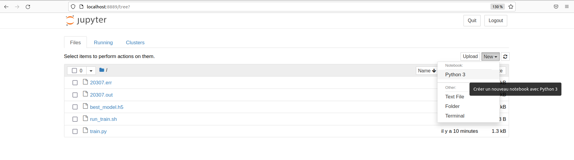
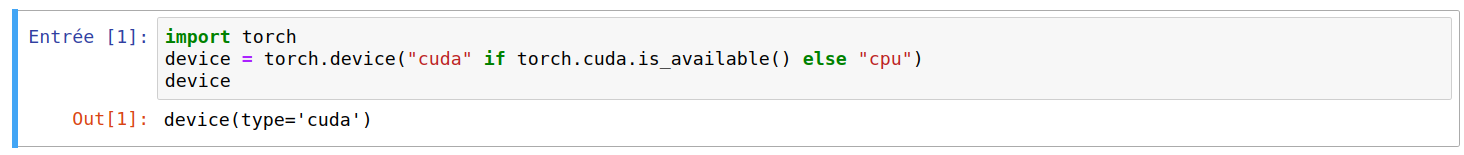
By putting the following code in a code cell and executing it,
import tensorflow as tf
from tensorflow.python.client import device_lib
print("GPUs Available: ", tf.config.experimental.list_physical_devices("GPU"))
import torch
device = torch.device("cuda" if torch.cuda.is_available() else "cpu")
device
we should get :
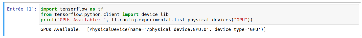
If the displayed list is not empty, then TensorFlow has successfully detected the GPU and will use it to speed up its calculations throughout the rest of the Jupyter Notebook code.
If the device type is cuda, then PyTorch has detected the GPU and will use it to speed up its calculations throughout the rest of the Jupyter Notebook code.
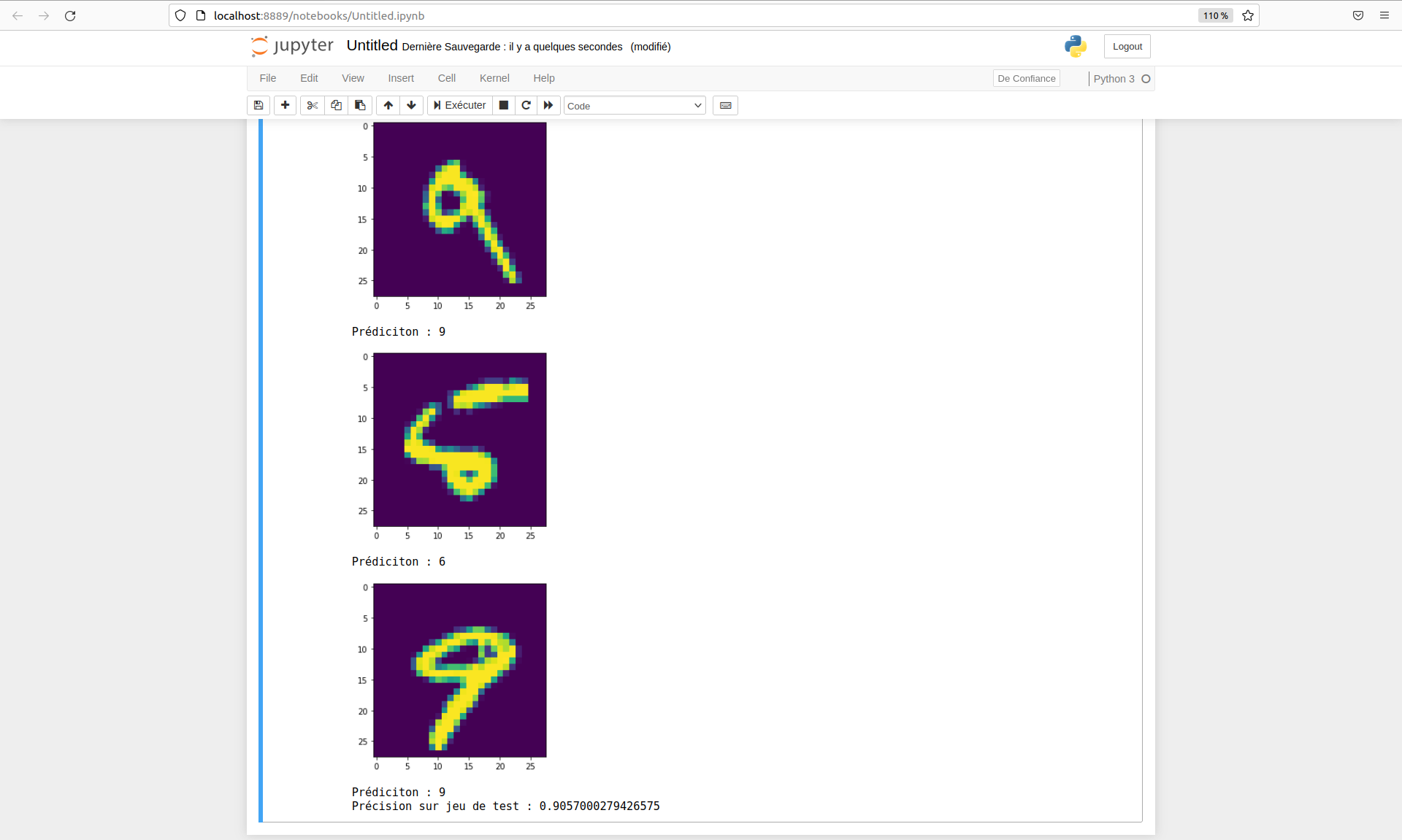
Finally, the code below allows to load the model, to evaluate it on a test set and to visualize some predictions.
from tensorflow.keras.datasets import mnist
from tensorflow.keras.utils import to_categorical
import matplotlib.pyplot as plt

%matplotlib inline

(X_train, y_train), (X_test, y_test) = mnist.load_data()
num_test   = X_test.shape[0]
img_height = X_train.shape[1]
img_width  = X_train.shape[2]
X_test  = X_test.reshape((num_test, img_width * img_height))
y_test = to_categorical(y_test, num_classes=10)

model = tf.keras.models.load_model("best_model.h5")

loss, metric = model.evaluate(X_test, y_test, verbose=0)

y_pred = model(X_test)

for i in range(10):
    plt.figure()
    plt.imshow(X_test[i].reshape((img_width, img_height)))
    plt.show()
    print(f"Prédiciton : {tf.math.argmax(y_pred[i])}")

print(f"Précision sur jeu de test : {metric}")
from torchvision import datasets, transforms
import matplotlib.pyplot as plt

from train import Classifier

%matplotlib inline

transform=transforms.Compose([
        transforms.ToTensor(),
        torch.squeeze,
        torch.flatten
])

dataset = datasets.MNIST("data", train=False, download=True, transform=transform)

model = torch.load("best_model.pt").to(device)

test_loader = torch.utils.data.DataLoader(dataset, batch_size=1)

model.eval()
accuracy = 0
with torch.no_grad():
    for i, (X, Y) in enumerate(test_loader):
        X, Y = X.to(device), Y.to(device)
        y_pred = model(X)
        y_classes = torch.argmax(y_pred, dim=1)
        accuracy += torch.sum(y_classes == Y)

        if i < 10:
            plt.figure()
            plt.imshow(X[0].reshape(28, 28).cpu())
            plt.show()
            print(f"Prédiction : {y_classes[0].item()}")
    accuracy = accuracy.item()/len(test_loader.dataset)
print(f"Précision sur jeu de test : {accuracy}")
Here is an example of the results obtained:
Alternatives
In this tutorial, we have run the training via a submission script and the model operation with a Jupyter Notebook via an interactive job, however:
- it is also possible to run the training via an interactive job, which can be useful for testing your training program on a development-only compute node.
- similarly, it is possible to perform model exploitation via a submission script. This can be useful to generate predictions immediately after the training. The code to be executed should therefore be in a .py file and its execution should be specified in the run_train.sh file.